Beyond Elo, Part I: The Core Rating Model

The first major problem was simple: a Blood Bowl result is not only evidence about the coach, but also about the roster being used.

If coach strength and roster strength are both affecting the result, a useful rating model needs some way to separate them. It also needs to know how confident it should be in each estimate, and it needs to predict wins, draws, and losses directly.

Those requirements led to the core model developed in this article: Davidson three-outcome probabilities, separate Coach Rating and Roster Rating states, and uncertainty-aware updates.

Later parts build on that foundation by adding persistent draw tendency and, where team-value data exists, roster strength that varies with TV and an additional TV matchup effect.

A three-outcome game needs a three-outcome model

Traditional Elo is usually expressed through an expected score:

• win = 1
• draw = 0.5
• loss = 0

That is useful for updating ratings, but it is not quite the question a predictor needs to answer.

For prediction, I want three probabilities:

$$P(\text{win}),P(\text{draw}),P(\text{loss}).$$

For that I use a Davidson model, which extends the paired-comparison framework by treating the draw as a genuine third outcome.

If the pregame strength difference is $D$, define

$$x=\frac{\ln 10}{2F}D,$$

where $F$ is the fixed scale that converts a rating gap into the probability curve. Let $U$ be the fixed draw term used by the core model in this article. Part II later introduces a baseline $U_0$ and allows the game-specific $U$ to vary with draw tendency. Then

$$P(W)=\frac{e^x}{e^x+e^{-x}+U},$$$$P(L)=\frac{e^{-x}}{e^x+e^{-x}+U},$$$$P(D)=\frac{U}{e^x+e^{-x}+U}.$$

The practical advantage is straightforward: the model predicts all three possible results directly, while also making close matchups naturally more draw-prone and reducing draw probability as the strength mismatch grows. That gave me a better foundation than ordinary Elo, but it still left the larger problem of separating coach strength from roster strength.

The first big problem: one number was doing too much

The original instinct was to rate coaches, but that quickly creates a problem. The same coach can play one tournament with a strong roster and another with a weaker one, and a coach-only model has no explicit way to represent that difference. If results change systematically with roster choice, some of that effect has to be absorbed into the coach rating instead.

That is not what I want Coach Rating to represent, so the model separates coach strength from roster strength:

$$D=(C{R}_1-C{R}_2)+(R{R}_1-R{R}_2),$$

where $CR$ is Coach Rating and $RR$ is Roster Rating.

The model can then ask two separate questions:

How strong is this coach?

and

How strong is this roster, after accounting for who is coaching it?

That separation changes what the ratings mean. Roster Rating is not a win-rate table; it is inferred jointly with Coach Rating through the chronological sequence of games. Results provide evidence about both components, and the model has to determine how that evidence should be shared between them.

There are also games where one component provides no information at all. If both coaches use the same roster, the roster terms cancel, so the result can tell us about the coaches but not whether that roster is stronger or weaker than another.

Does Roster Rating actually mean anything?

If two coaches are rated about equally, does the coach using the higher-rated roster actually do better?

Using chronological pregame ratings from the NAF ranking, I selected games where the two coaches were within 25 CR of each other and grouped them by the RR advantage of the stronger-rated roster. Here, average result uses win = 1, draw = 0.5, and loss = 0.

RR advantage	Games	Higher-RR side W / D / L	Average result
0–20	16,663	37.8% / 25.3% / 36.8%	50.5%
20–50	20,904	40.5% / 25.0% / 34.5%	53.0%
50–100	17,351	43.9% / 24.9% / 31.3%	56.3%
100–150	6,362	50.4% / 23.7% / 25.9%	62.2%
150+	5,592	60.0% / 20.5% / 19.5%	70.3%

The higher-RR side had essentially no corresponding coach-rating advantage in those groups; its mean CR difference was slightly negative throughout. Tightening the coach match further to within 10 CR produced the same basic progression.

The pattern is exactly what we would expect if RR is capturing real differences in roster strength: with coach strength held roughly constant, larger RR gaps are associated with progressively better results for the higher-rated roster.

Ratings should know when they are uncertain

Another weakness of a simple Elo implementation is that update size is usually controlled by a fixed or externally chosen K-factor. But a newly observed coach or roster should not necessarily react to one result in the same way as a well-established one.

So each learned rating, an internal estimate rather than a directly observable quantity, carries both a current value and an uncertainty around that value. A poorly observed coach or roster starts uncertain and can move quickly; as evidence accumulates, uncertainty usually contracts and individual results normally have less influence. This is related in spirit to Glicko, but the uncertainty is attached separately to each learned coach and roster rating rather than only to one coach number. Figure 1 shows the uncertainty attached to the final BB2025 roster ratings.

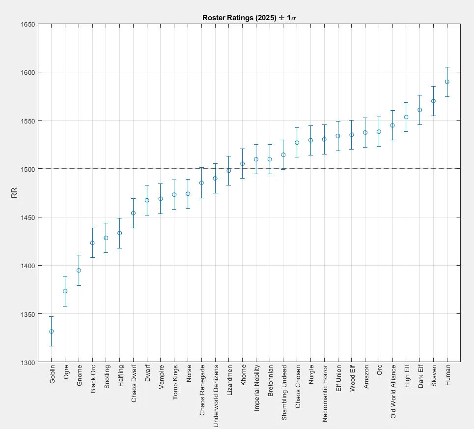
Figure 1. Final BB2025 Roster Rating estimates with ±1$\sigma$ uncertainty.

That uncertainty controls how strongly each latent state can respond to new evidence and how a game's correction is shared between coach and roster strength.

Uncertainty does not shrink forever, though. After each update, the model adds a small amount of uncertainty back to the evolving strength states, allowing for the possibility that underlying strength changes over time. Mature ratings therefore tend to settle around a nonzero uncertainty level rather than converging toward perfect certainty.

How one game updates the model

Before a game, the current CR and RR values determine the strength difference $D$. The Davidson model then produces the three outcome probabilities:

$$P(W),P(D),P(L).$$

For the strength update, define the observed score

$$S=\{\begin{array}{ll}1& \text{win}\\ 1/2& \text{draw}\\ 0& \text{loss}\end{array}$$

and the model's expected score

$$E=P(W)+\frac{1}{2}P(D).$$

The difference between what happened and what the model expected sets the direction of the strength update:

$$S-E.$$

So the basic logic is familiar from Elo:

• perform better than expected and strength moves upward;
• perform worse than expected and strength moves downward;
• perform about as expected and the movement is small.

The difference here is that the correction is not assigned to one rating with one fixed K-factor. Because coach and roster strength are separate uncertain states, the game distributes the correction between them according to their current uncertainties: a state the model is still unsure about can move more, while a well-established state moves less.

The uncertainty itself is updated as well. Early evidence usually makes ratings more stable and reduces the influence of later single-game results, until posterior contraction and process variance begin to balance.

Everything is chronological

One rule runs through the entire project:

A game must be predicted before its result is allowed to affect the model.

For every game:

1. read the current pregame states;
2. calculate the pregame strength and draw coordinates;
3. produce win, draw, and loss probabilities;
4. record the prediction;
5. observe the result;
6. update the latent states;
7. move to the next game.

That ensures a game's result cannot affect the ratings used to predict that game. Within each chronological replay, the prediction is recorded before the result updates any learned state.

The fixed model settings are chosen from historical data before a chronological replay begins, then held constant. Only the evolving coach and roster ratings update after each result is observed. You can see in Figure 2 how selected roster ratings move away from the common starting point and gradually settle as evidence accumulates.

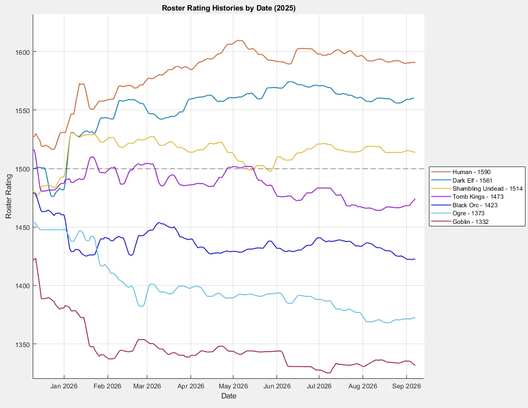
Figure 2. Selected BB2025 Roster Rating histories.

The fitting process rewards the model for assigning more probability to the result that actually happens, rather than merely naming the most likely winner. The primary fitting metric is Log Loss because the model is trying to produce good probabilities, not merely pick the most likely winner.

What Part I establishes

The core model treats Blood Bowl as a three-outcome prediction problem, separates coach strength from roster strength, and lets both evolve according to their uncertainty, with each game predicted before its result is allowed to update the model.

That establishes the strength side of the model. The next question is whether strength alone is enough to explain how often games end in draws. That is the subject of Beyond Elo, Part II: Learning Draw Tendency.

Explore the core model

In Analytics, use the predictor to see how coach and roster strength combine in a matchup. Coach and roster rankings, together with their rating histories, show the model states behind those predictions.

Technical reference

For the derivation behind this article, see Core Davidson Model.

Updates

Update, October 1, 2026: The uncertainty and chronological-update sections were clarified after a follow-up audit. The model itself is unchanged, but earlier wording overstated what final roster-uncertainty differences can demonstrate about roster-specific learning rates.