Appearance
Beyond Elo, Part III: When Roster Strength Depends on Team Value
The core prediction model begins by giving each roster a single strength rating. That is a useful starting point, but team value eventually exposes the limit of that simplification.
If a roster becomes stronger or weaker as a team develops, then one fixed RR is not enough. A 1100k TV team and an 1800k TV team using the same roster may not represent the same underlying roster strength.
But even that does not capture everything. After allowing roster strength itself to vary with team value, there may still be an additional effect from the difference in TV between the two teams entering the match.
That creates two separate questions:
How strong is this roster at its current team value?
Is there an additional matchup effect from the TV difference between the two sides?
Working out how to separate those effects became one of the longest parts of the project.
The result is a team-value extension of the predictor, using additional information that is already known before kickoff.
On FUMBBL, this richer TV-dependent roster model is used for official rosters; custom rosters keep the single Roster Rating from the core model.
A single roster rating was not enough
The core model gives every roster its own strength rating:
That is already a large improvement over a coach-only system because the model no longer has to force roster strength into the coach rating.
But it still assumes something strong:
a roster has the same strength at every team value.
That is not obviously true in Blood Bowl.
Some rosters gain a lot from additional skills and players. Others reach much of their practical strength earlier. Some become more efficient at particular development ranges. Some may be relatively strong at low TV and less exceptional later, or the other way around.
So the next question became:
Can roster strength itself be allowed to vary with team value?
From one RR to a strength curve
Instead of giving a roster one fixed strength value, this extension estimates its strength at several anchor TV levels, called control points. The roster's strength at the actual pregame TV is then interpolated between those points.
Conceptually, instead of thinking of RR as one number per roster,
it is better to think of roster strength as a function of team value:
The model learns how strong a roster appears to be at different stages of team development.
That means a 1100k TV Human team and a 1800k TV Human team no longer have to inherit exactly the same roster contribution merely because both are Humans.
The Vampire curve in Figure 1 makes the idea concrete. The circles are the learned control points, while the line shows the interpolated roster strength between them. The uncertainty band shows how much uncertainty remains around the estimated roster strength across team value.
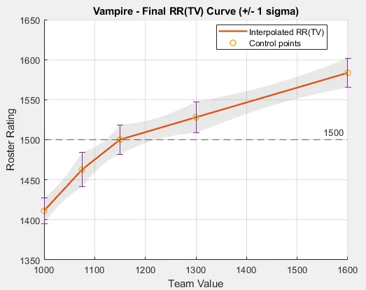
Figure 1. Final Vampire RR(TV) curve with uncertainty.
Here, roster strength clearly changes across team value rather than remaining fixed at one RR.
The same curve can also be followed through time. Figure 2 places team value along one axis, roster updates along another, and the height of the surface is the roster's current learned strength at that TV. You do not need to read every detail of the surface. The important point is that its shape is not pre-set: it develops from game evidence as the model learns.
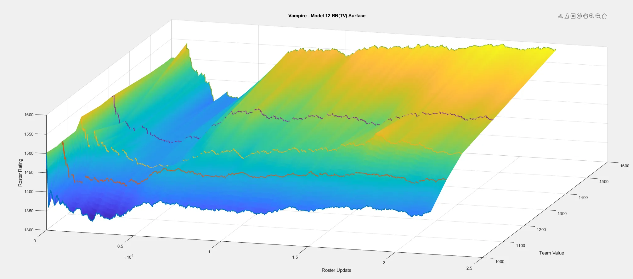
Figure 2. Vampire RR(TV) surface across team value and roster updates.
As games are observed, different TV ranges can settle at different strength levels.
One roster may gain strength quickly over a certain TV range, while another changes much less. A roster can therefore be relatively strong in one development range and less exceptional in another.
That is what
The uncertainty has to move with the curve
Once roster strength became a function of team value, its uncertainty had to follow the same structure.
Each control point has its own estimated strength and uncertainty. Between two points, the model derives the uncertainty from the uncertainties of the active control points and their interpolation weights, so the uncertainty band remains tied to the same latent states that define the strength curve.
What happens after one game?
Suppose a roster plays at a team value between two control points. Only those active points contribute to the current (RR(TV)), so the game should mainly teach the model about that part of the curve.
The game mainly updates the nearby points on that roster's strength curve, especially where the model remains uncertain. This makes learning local. A game played around one TV should mostly refine roster strength around that part of the development curve, rather than shifting the entire curve everywhere at once.
Earlier versions let learning about one part of the curve propagate too far, sometimes producing large movements elsewhere. The final approach deliberately keeps learning local:
Learn mainly from the part of the curve that was actually observed.
The control-point histories in Figure 3 make that local behaviour easier to see. Each TV point follows its own trajectory rather than the entire roster curve moving as one block. The model can therefore learn differently from games played at different stages of team development.
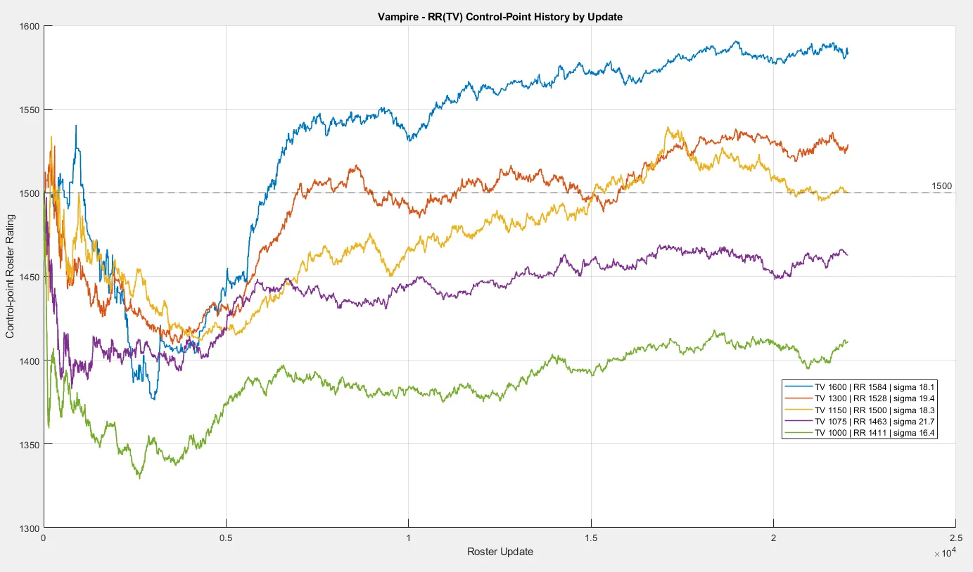
Figure 3. Vampire RR(TV) history showing local curve evolution.
The Vampire history also shows a useful real-world transition: the change associated with the new Vampire roster introduced under the 2020 rules is visible in the trajectories rather than being hidden inside one scalar roster rating.
But RR(TV) did not explain everything
At this point, the model already separated coach strength from roster strength, allowed roster strength to vary with team value, and carried uncertainty through the relevant latent states.
Residual analysis still showed a clear pattern with team-value difference. After accounting for coach strength and (RR(TV)), teams with a TV advantage tended to outperform the model, while teams with a TV disadvantage tended to underperform it. Figure 4 shows the remaining result imbalance after the model's prediction: values above zero mean the TV-advantaged side did better than expected, while values below zero mean it did worse.
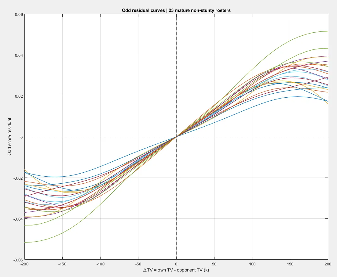
Figure 4. Directional residual structure by team-value difference for mature non-stunty rosters.
Each coloured line represents one mature non-stunty roster. The exact shape of any individual line is not the important part. Across many rosters, the lines show the same broad directional pattern, with the effect generally growing as the TV gap widened.
That pointed to a second TV effect, distinct from the roster's own strength curve.
(RR(TV)) asks:
How strong is this roster at this team value?
Delta TV asks:
Does the difference in team value between the two sides add an extra matchup effect?
A roster can become stronger as its own TV increases, while a separate advantage can still come from entering a particular match with more TV than the opponent.
The model therefore needed to represent both.
Delta TV as a matchup effect
The extended strength coordinate becomes
with
The coach and roster terms are learned ratings that update according to their uncertainty. The delta-TV term plays a different role: it is a deterministic pregame correction based on the observed difference in team value.
That correction is applied before the game is predicted, but it does not have its own latent state or uncertainty. CR and RR are then updated from whatever part of the result remains unexplained after the TV mismatch has already been accounted for.
Keeping those roles separate helps prevent a systematic TV-gap effect from being absorbed into coach or roster strength.
The shape of the TV effect was fitted from the residual structure
There was no good reason to assume that 100 TV of advantage should always mean exactly twice as much as 50 TV. Instead, the shape was guided by the residual structure left by the (RR(TV)) model.
A flexible fitted curve captured the central pattern well. Farther into the supported TV gaps, however, its first version returned toward zero while the observed effect remained visible. Figure 5 compares the empirical common shape with that initial fitted behaviour.
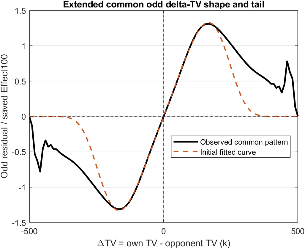
Figure 5. Empirical common delta-TV residual shape compared with the initial fitted curve.
That exploratory fit helped determine the functional form, but it is not the final production correction. The final function was refitted jointly with the rest of the model during the full chronological replay. Over the practical range of observed TV differences:
- the effect has the correct sign;
- a larger TV advantage generally produces a larger strength correction;
- the marginal gain becomes smaller as the difference grows;
- the function is symmetric under swapping the two teams;
- equal TV gives exactly zero correction.
For readers who want the precise mathematical definition, the final correction combines a central fitted shape with a persistent tail term:
Stunty teams were different
The delta-TV effect did not generalize consistently to stunty games, so the final model does not force the same correction onto them. Whenever either side uses one of the designated stunty rosters, the delta-TV matchup term is simply disabled.
The rest of the model works exactly as before. Only the additional TV-gap correction is removed.
Putting the TV extension together
In short, (RR(TV)) describes the roster's own strength at its current stage of development, while
As in the core model, both team values are read before kickoff and the prediction is recorded before the result can update any rating. Part I explains that chronological rule in full.
The development was messier than the final equations
The TV extension followed the same development rule described in the overview: retain only structure that continued to explain a repeatable failure of the simpler model.
Several development steps led here. Earlier curve-learning approaches moved roster strength too broadly across the TV curve. The first fitted delta-TV shape worked well in the centre but returned toward zero in the tails while the empirical effect remained. Other approaches produced unstable shapes or fitted parameters that kept running into degenerate limits. Some improved Log Loss while still behaving in ways that were difficult to justify.
The useful breakthrough was separating the problem into two questions: first, whether roster strength itself changes with TV, and then whether a separate matchup effect remains after that is accounted for.
That is how (RR(TV)) and the delta-TV correction emerged. Each survived because it explained systematic structure that simpler versions kept leaving behind.
Explore team value
The live implementation powers the corresponding ratings, histories, and matchup analysis tools on Analytics.
In the FUMBBL Analytics view, use the predictor to see how team value changes a specific matchup. Roster rankings at different TV points and roster histories show the learned development patterns behind those predictions.
Technical references
For the mathematics behind this extension, see Roster Strength by Team Value and Delta-TV Matchup Correction. The shared prediction model is documented in Core Davidson Model.
Updates
Update, October 1, 2026: Clarified the official-roster scope of the TV-dependent model, and distinguished the exploratory residual-space fit from the final production delta-TV correction.